How Syntitan’s data preparation improved Logistic Regression’s F1 on the UCI Iranian Churn dataset—with the same model settings.
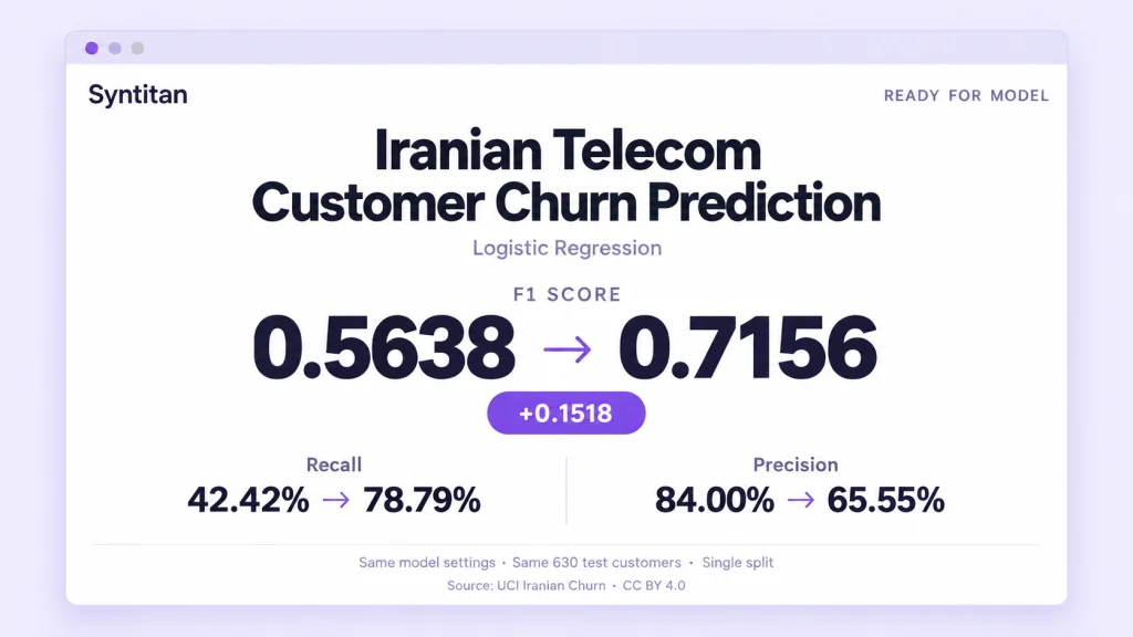
Customer churn prediction helps telecom teams identify customers who may leave. Using the UCI Iranian Churn dataset, we tested how Syntitan’s data preparation changed Logistic Regression performance while keeping the model settings fixed. F1 increased from 0.5638 to 0.7156 on the same 630 evaluation records.
Logistic Regression initially detected 42 of the 99 churners in the evaluation set. After data preparation, it detected 78. Recall rose from 42.42% to 78.79%.
The additional detections came with more false alarms: 41 non-churners were incorrectly flagged, compared with 8 before preparation. The result offers a concrete example of how changing the data can change a model’s usefulness—and why the full comparison matters.
The Iranian Telecom Dataset for Customer Churn Prediction
The UCI Iranian Churn dataset contains 3,150 customer records and 13 input features from an Iranian telecommunications company.
The features describe customer activity and account characteristics, including call failures, complaints, subscription length, call and SMS usage, tariff plan, and customer value. The target column, Churn, indicates whether a customer left.
According to UCI’s documentation, the input attributes summarize the first nine months of activity. The churn labels describe customer status at the end of month twelve, leaving a three-month planning gap.
This makes the task relevant to retention planning: use earlier customer information to identify who may leave later. Our experiment measures prediction performance; it does not test whether contacting those customers would prevent churn.
Customer Churn Prediction with the Same Model Settings
We used Syntitan’s Ready for Model workflow to compare performance before and after data preparation.
For each model, we kept the model settings fixed and retrained it separately on the original and prepared training data. Both versions were evaluated on the same 630 original customers:
- 99 customers who churned.
- 531 customers who did not churn.
The classification threshold remained at 0.5. The original training split contained 2,520 rows; the prepared training data for Logistic Regression and Random Forest contained 3,035.
We then reran the exported Proof Kit scripts for both models and reproduced their reported results.
| Metric | Logistic Regression: before | Logistic Regression: after | Random Forest: before | Random Forest: after |
|---|---|---|---|---|
| F1 | 0.5638 | 0.7156 | 0.8808 | 0.8911 |
| Recall | 0.4242 | 0.7879 | 0.8586 | 0.9091 |
| Precision | 0.8400 | 0.6555 | 0.9043 | 0.8738 |
| ROC-AUC | 0.9208 | 0.9399 | 0.9875 | 0.9892 |
| Average precision¹ | 0.7563 | 0.8144 | 0.9256 | 0.9283 |
| Accuracy | 0.8968 | 0.9016 | 0.9635 | 0.9651 |
¹Shown as PR-AUC in the interface; the exported script calculates average precision.
These results come from one train/test split, with 99 churners in the evaluation set. They describe this experiment; repeated evaluation would be needed to determine how consistently the gains hold.
Logistic Regression: 36 more churners identified
Logistic Regression showed the larger improvement. Its F1 increased by 0.1518, from 0.5638 to 0.7156.
F1 combines precision and recall. Here, the increase reflects a substantial gain in recall alongside a decline in precision.
| Prediction outcome | Before preparation | After preparation |
|---|---|---|
| Churners correctly identified | 42 | 78 |
| Churners missed | 57 | 21 |
| Non-churners incorrectly flagged | 8 | 41 |
| Non-churners correctly classified | 523 | 490 |
Before preparation, the model missed more than half of the churners. After preparation, it identified nearly four in five.
For a retention team, however, the resulting contact list would also be larger. The model flagged 50 customers before preparation and 119 afterward. It found 36 additional churners while adding 33 false positives.
That distinction matters when choosing how to act on predictions. A low-cost reminder and an expensive retention offer have different consequences when sent to someone who was unlikely to leave. The experiment makes the change in predictions visible; the business must still assess the value of acting on it.
Did the model become better at ranking customers?
A model can identify more churners simply by flagging more people. That is why we also examined metrics that evaluate predicted scores across thresholds.
For Logistic Regression, ROC-AUC increased from 0.9208 to 0.9399, and average precision increased from 0.7563 to 0.8144.
These results indicate improved ranking performance on this evaluation set, alongside the higher F1 at the fixed threshold. The observed change therefore extends beyond the number of positive predictions alone.
We did not compare the prepared-data model against threshold tuning or class weighting on the original data. Those remain useful comparisons before deciding which approach best fits a retention workflow.
Random Forest: higher final performance, less room to improve
Random Forest started from a stronger baseline. Its original F1 of 0.8808 was already higher than Logistic Regression’s score after preparation.
After preparation, Random Forest’s F1 increased to 0.8911. It identified 90 of the 99 churners, compared with 85 before.
| Prediction outcome | Before preparation | After preparation |
|---|---|---|
| Churners correctly identified | 85 | 90 |
| Churners missed | 14 | 9 |
| Non-churners incorrectly flagged | 9 | 13 |
| Non-churners correctly classified | 522 | 518 |
The change was modest: five additional churners identified, four additional false positives, and one fewer classification error overall. A paired accuracy test did not establish a statistically significant difference; that test does not directly test the F1 change.
The comparison makes the trade-offs of each preparation approach visible. Logistic Regression showed the larger F1 increase, while Random Forest delivered the higher final F1. Both are relevant when deciding what to evaluate next.
What Syntitan changed
The preparation summary lists feature generation and minority-class augmentation for both models, with an additional LLM-based feature-generation step for Logistic Regression. The Random Forest interface identifies binning and row augmentation among the applied refinements.
These steps change the information available during training and how it is represented. In this experiment, the prepared training datasets contained 515 more rows than the original training split.
The exported split metadata assigns the additional training records outside the evaluation set. Both sides of the comparison use the same original test customers.
The export supports reproducing model training and scoring from the prepared datasets. It does not fully document the augmentation algorithm or independently establish how every upstream feature-generation decision was fitted. A complete preparation audit would require those additional details.
From a performance chart to an inspectable result
Syntitan’s Proof Run presents the before-and-after comparison. The downloadable Proof Kit provides the files needed to examine it further.
For the two runs discussed here, those files included the original and prepared datasets, model execution scripts, and split metadata. Running the scripts reproduced the metrics and generated predicted probabilities for further inspection.
That let us check the practical meaning of the headline result:
- Were both models evaluated on the same customers?
- How many additional churners were identified?
- How many additional false positives appeared?
- Did ranking metrics improve alongside F1?
For teams evaluating data preparation, this makes the result easier to assess and share. The discussion can move from a score on a screen to the predictions and evaluation setup behind it.
What this means for customer churn prediction
On this Iranian telecom dataset, Syntitan’s data preparation increased Logistic Regression’s F1 from 0.5638 to 0.7156 with the same model settings. The model identified 78 of 99 churners, up from 42, while generating more false positives.
Random Forest showed a smaller improvement and retained the stronger final score.
The practical value is having a concrete comparison before committing to a preparation approach. Teams can examine the change in detection, precision, and ranking performance, then evaluate whether that balance suits their task.
For this experiment, the next step is to test whether the results hold across repeated splits and compare them with threshold and class-weight adjustments. Retention campaign costs, prevented churn, revenue impact, and workflow time were not measured.
Dataset attribution: Iranian Churn, UCI Machine Learning Repository (2020), licensed under CC BY 4.0. DOI: 10.24432/C5JW3Z.