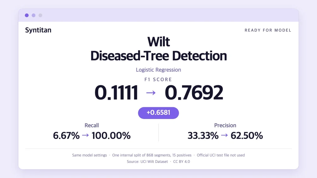
The same logistic regression configuration detected one diseased-tree segment before data preparation and 15 afterward.
In this UCI Wilt Dataset experiment using Syntitan’s Ready for Model workflow, logistic regression scored an F1 of 0.1111 before data preparation and 0.7692 afterward on the same internal evaluation split. Recall and precision both increased. False positives also rose, from two to nine.
The scale of the evaluation matters: these results come from one internal split containing 868 image segments, including only 15 positives. We used the original training file, not the dataset’s separate official test file. This is an exploratory comparison, not evidence of deployment performance across forests or satellite images.
Key takeaways
- Logistic regression F1 rose from 0.1111 to 0.7692 with the same settings: 14 more diseased-tree segments detected, with seven more false positives.
- All four models recorded higher F1 in this split. XGBoost reached the highest final F1, 0.9032, with fewer false positives than its baseline.
- Random Forest shows why F1 alone is incomplete: recall rose, but precision, ROC-AUC, and average precision fell.
- The evaluation has only 15 positives, and no McNemar p-value falls below 0.05, so this is an exploratory result, not a significance claim.
What the UCI Wilt Dataset contains
The UCI Wilt Dataset contains tabular features extracted from QuickBird satellite imagery for diseased-tree detection. Each row represents an image segment, rather than an individual tree or a raw satellite image.
The target is class: w denotes diseased trees, while n denotes all other land cover. The negative class should therefore not be described simply as healthy trees. The five inputs describe green, red, and near-infrared values alongside panchromatic texture and variation.
UCI distributes separate training.csv and testing.csv files. The baseline in this experiment matches the 4,339-row training file in both feature values and labels: 74 positive segments and 4,265 other-land-cover segments. The separate 500-row test file was not used.
How the evaluation was set up
All four models started from the same baseline table and used the same original evaluation-row positions. The exported split allocated 3,471 original rows to training and 868 to evaluation. The training set contained 59 positives; evaluation contained 15 positives and 853 negatives.
Within each model’s comparison, its configuration and the default 0.5 prediction threshold stayed fixed. The model was retrained separately on the before and after training data. Prepared evaluation rows represent the same original records, with the corresponding feature transformations applied.
Preparation differed by model. This is a set of four before-and-after comparisons, not an experiment in which one common prepared dataset was supplied to all four classifiers. Differences between their final scores reflect both the model and its preparation.
Logistic regression: higher recall and precision, with more false positives
| Metric | Before | After |
|---|---|---|
| F1 | 0.1111 | 0.7692 |
| Precision | 0.3333 | 0.6250 |
| Recall | 0.0667 | 1.0000 |
| ROC-AUC | 0.9860 | 0.9988 |
| Average precision | 0.5166 | 0.9036 |
| True positives | 1 | 15 |
| False negatives | 14 | 0 |
| False positives | 2 | 9 |
| True negatives | 851 | 844 |
The absolute F1 gain was 0.6581. All 15 positive evaluation segments were detected after preparation, compared with one before. That recovered 14 missed cases at the cost of seven additional false positives.
Precision increased because the composition of flagged records improved: before preparation, one of three flagged segments was positive; afterward, 15 of 24 were positive. A rise in precision does not mean the absolute false-positive count fell.
The baseline already had a high ROC-AUC of 0.9860 despite weak recall at the default threshold. This makes a validation-selected threshold or class-weight baseline an important missing comparison. The prepared version also improved ROC-AUC and average precision, but we have not isolated the contribution of each preparation step.
One positive evaluation case changes recall by approximately 6.67 percentage points. The observed 1.0000 recall therefore should not be presented as a guarantee of complete disease detection. Repeated evaluation and testing on independent imagery are needed to assess stability and generalization.
All four models improved F1 in this split
All four scripts were rerun. Arrows show before → after for positive-class metrics.
| Model | F1 | Precision | Recall |
|---|---|---|---|
| Logistic Regression | 0.1111 → 0.7692 | 0.3333 → 0.6250 | 0.0667 → 1.0000 |
| Random Forest | 0.8000 → 0.8750 | 1.0000 → 0.8235 | 0.6667 → 0.9333 |
| LightGBM | 0.8276 → 0.8667 | 0.8571 → 0.8667 | 0.8000 → 0.8667 |
| XGBoost | 0.8000 → 0.9032 | 0.8000 → 0.8750 | 0.8000 → 0.9333 |
XGBoost achieved the highest final F1. It detected 14 positive segments instead of 12, while reducing false positives from three to two. Logistic regression showed the largest F1 increase, but did not become the best-performing model.
For completeness, the confusion counts below use TN / FP / FN / TP order.
| Model | Before (TN / FP / FN / TP) | After (TN / FP / FN / TP) |
|---|---|---|
| Logistic Regression | 851 / 2 / 14 / 1 | 844 / 9 / 0 / 15 |
| Random Forest | 853 / 0 / 5 / 10 | 850 / 3 / 1 / 14 |
| LightGBM | 851 / 2 / 3 / 12 | 851 / 2 / 2 / 13 |
| XGBoost | 850 / 3 / 3 / 12 | 851 / 2 / 1 / 14 |
Random Forest illustrates why F1 alone is incomplete: its recall increased, but precision declined as false positives rose from zero to three. Its ROC-AUC also decreased from 0.9995 to 0.9991, and average precision fell from 0.9768 to 0.9641. Its F1 improvement at 0.5 therefore does not establish improved ranking performance.
What changed in the data
| Model | Preparation described in the export | Training rows | Input features after preparation |
|---|---|---|---|
| Logistic Regression | Generated features, outlier treatment, distribution transformation, binning, and augmented training data | 3,471 → 4,651 | 42 |
| Random Forest | Feature selection and minority augmentation; all five source features remain in the exported table | 3,471 → 4,651 | 5 |
| LightGBM | Outlier treatment and minority augmentation | 3,471 → 4,651 | 5 |
| XGBoost | Generated features and feature selection | 3,471 → 3,471 | 20 |
The logistic regression export includes spectral ratios, interactions, differences, indicators, and binned features. For example, it includes red-to-green and near-infrared-to-green ratios. XGBoost uses a selected set of original and derived features.
For logistic regression, Random Forest, and LightGBM, the prepared training block contains 1,239 positives and 3,412 negatives. That is a net addition of 1,180 positive training rows. XGBoost retains 59 positives and 3,412 negatives. No augmented rows are intended for evaluation under the exported split layout.
The files document the resulting tables and broad preparation categories. They do not include enough upstream generation code to reconstruct the exact augmentation algorithm, fitted transformations, or feature-selection process. The final feature counts are verified from the CSVs; the preparation-stage descriptions are export metadata.
What the verification kit lets you check
The ZIP contains a shared README and one folder per model: Logistic Regression, Random Forest, LightGBM, and XGBoost. Each folder includes the following files.
| File | What to check |
|---|---|
data_before.csv | Inspect the baseline feature table and class labels. |
data_after.csv | Inspect the prepared data for that model, including its features and row counts. |
proof_split.json | Read the train/test block boundaries and original evaluation-row positions. |
run_model.py | Retrain both versions and recompute the metrics and confusion counts. |
We checked that the four baseline tables match, that evaluation positions are shared across models, and that the prepared test-block labels align with the original labels. These checks support a paired comparison. They do not independently establish that every upstream transformation and preparation-selection step was fitted using training data only.
Proof kit: UCI Wilt Dataset
ZIP · 2.0 MB · 4 model folders
- Before and after datasets for each model
- A standalone
run_model.pyscript per model - Split information (
proof_split.json) in every model folder
Reruns model training and scoring; it does not rerun the upstream preparation steps. Data: UCI Wilt Dataset, CC BY 4.0, prepared derivatives.
How to rerun a comparison from the kit
- Install the packages.
pip install pandas numpy scipy scikit-learn lightgbm xgboost - Enter a model folder.
cd 'Logistic Regression' - Run the script.
python run_model.py, then repeat from the other model folders to compare all four models.
The script prints the scores and creates a metrics JSON file containing nine metrics, confusion counts, class-specific results, split information, ground-truth labels, and predicted probabilities. The pr_auc field is average precision, computed with average_precision_score; it is not trapezoidal integration of the precision-recall curve.
These outputs allow you to reconstruct curves and inspect predictions. The kit reproduces training and scoring from the exported CSVs, rather than the entire preparation process from satellite imagery. Our rerun used scikit-learn 1.8.0, LightGBM 4.7.0, and XGBoost 3.4.1; the split seed is 42. Package versions should be recorded because the kit does not provide a pinned environment lockfile.
How to read the statistical results
The script calculates a separate McNemar p-value for each model’s before-and-after predictions: 0.2100 for logistic regression, 1.0000 for Random Forest, 1.0000 for LightGBM, and 0.3750 for XGBoost. These are unadjusted values, and none falls below 0.05.
McNemar compares paired correctness, not F1 directly. The results do not establish statistically significant improvements in paired correctness at that cutoff, and a non-significant result does not prove that the two versions are equivalent. We make no claim of statistically significant F1 improvement.
The next checks are repeated splits, validation-selected thresholds and class weights, and an untouched final evaluation set. Using the official test file would require applying transformations fitted only on training data, rather than fitting preparation anew on the test file. Spatially separated imagery would provide stronger evidence of transfer beyond the source image; the supplied table does not establish spatial independence.
What this experiment says about Ready for Model
This experiment shows measurable differences when the model configuration is held fixed and its prepared input changes. Logistic regression recovered substantially more positive segments in this split, while XGBoost achieved the highest final F1 with fewer false positives than its baseline.
The practical value of Syntitan here is an inspectable comparison: model-specific prepared data, the same original evaluation records, and runnable scoring code. The numbers support further testing of these preparation approaches. Forest-level disease prevalence, field inspection costs, operational savings, and end-to-end preparation time were not measured.
Related experiments with the same before-and-after setup: UCI Bank Marketing dataset, UCI Iranian Churn dataset, UCI Polish Companies Bankruptcy dataset, and UCI Shill Bidding Dataset.
Try it on your data. Syntitan Ready for Model runs the same kind of comparison: the same model settings, before and after data preparation, scored on the same evaluation records, with exported files for rerunning model training and scoring.
Dataset attribution: Johnson, B. (2013). Wilt [Dataset]. UCI Machine Learning Repository. https://doi.org/10.24432/C5KS4M. Licensed under CC BY 4.0. Prepared derivatives were used in this experiment; this does not imply endorsement by UCI or the dataset creator.