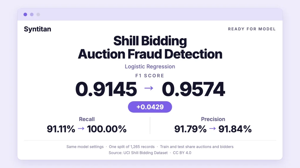
On the same 1,265 evaluation records, the model found 12 positive cases it had missed before. False positives rose by one, and precision stayed nearly the same.
In this UCI Shill Bidding Dataset experiment, Syntitan’s prepared data increased logistic regression F1 from 0.9145 to 0.9574 at the default 0.5 decision threshold. Recall rose from 0.9111 to 1.0000, while precision increased slightly from 0.9179 to 0.9184. True positives increased from 123 to 135; false positives increased from 11 to 12. Higher precision and a higher false-positive count can occur together, because precision measures the proportion of flagged records that are actually positive.
The other three models tell a different story: their F1 scores did not improve, and all three already outperformed the prepared logistic regression model. That makes this a useful example of where data preparation helped a particular model, and where the baseline was already strong.
Key takeaways
- Logistic regression F1 rose from 0.9145 to 0.9574 with the same settings: 12 more positive records detected, with one more false positive.
- Precision rose slightly while the false-positive count grew, because precision is a proportion of flagged records, not a count of false alarms.
- Random Forest, LightGBM, and XGBoost did not change and still scored higher than the prepared logistic regression.
- The result comes from one split with 135 positives, and most test auctions and bidders also appear in training, so it is not yet a test on unseen auctions.
What the UCI Shill Bidding Dataset measures
The UCI Shill Bidding Dataset contains labeled records derived from eBay auctions. Shill bidding involves bids intended to inflate an auction price rather than make a legitimate purchase. The classification task distinguishes normal bidding from the dataset’s positive class.
The input files used here contain 6,321 rows: 5,646 normal records and 675 positive records, or approximately 10.68% positive. There are 13 columns including the target, three identifiers, and nine behavioral attributes. This is a prepared tabular benchmark, rather than raw auction event logs.
Behavioral attributes cover patterns such as successive outbidding, early and late bidding, bidder tendency, and winning ratio. Because some attributes depend on auction progress or historical outcomes, this experiment does not establish that the same inputs would be available at an early, real-time intervention point.
Results: higher recall, nearly unchanged precision
The logistic regression classifier and its settings stayed the same. Each version was retrained on its corresponding training data, and both were scored on the same original evaluation records.
| Metric | Before | After |
|---|---|---|
| F1 | 0.9145 | 0.9574 |
| Precision | 0.9179 | 0.9184 |
| Recall | 0.9111 | 1.0000 |
| ROC-AUC | 0.9964 | 0.9993 |
| Average precision (PR summary) | 0.9572 | 0.9938 |
| True positives | 123 | 135 |
| False negatives | 12 | 0 |
| False positives | 11 | 12 |
| True negatives | 1,119 | 1,118 |
Precision is TP / (TP + FP). Before preparation, 123 of the 134 flagged records were positive: 123 / 134 = 0.9179. After preparation, 135 of the 147 flagged records were positive: 135 / 147 = 0.9184. The model therefore detected more positive records while slightly improving the proportion of correct positive predictions, even though the absolute number of false positives rose by one.
Precision should also be distinguished from the false-positive rate, FP / (FP + TN). Among the same 1,130 normal records, that rate increased from 11 / 1,130 (0.97%) to 12 / 1,130 (1.06%). The result supports improved recall and slightly higher precision; it does not support a claim of fewer false alarms.
The absolute F1 increase was 0.0429. The prepared version detected all 135 positive records in this evaluation set, while flagging 12 of the 1,130 normal records. A recall of 100% describes this sample; it is not a claim that the model will catch every fraudulent case in production.
ROC-AUC and average precision also increased. The observed improvement therefore extends beyond the predictions at a single threshold. However, the experiment does not isolate which preparation step caused the gain, and it does not compare against a baseline tuned with class weights or a validation-selected threshold.
The evidence is one evaluation split with only 135 positives. Auction IDs overlap with training for 1,259 of the 1,265 test rows; bidder IDs overlap for 1,193. These are row-level results, not a test of generalization to entirely unseen auctions or bidders. A grouped or temporal evaluation is needed before making that claim.
What changed in the model input
The exported logistic regression table expanded from 13 to 58 columns. Added columns include behavioral interactions, logarithmic features, binary indicators, and binned features. For example, the export includes interactions between successive outbidding and winning ratio, and between bidding activity and auction duration.
The training block increased from 5,056 to 6,452 rows. Its positive-class count rose from 540 to 1,936, while the negative count stayed at 4,516: a net addition of 1,396 positive training rows. The evaluation block remained 1,265 rows. The export describes training-only row augmentation, but does not include enough generation code to independently reconstruct its exact sampling method.
There is also an important caveat about identifiers. The scoring script removes the original Record_ID, but retains Auction_ID and Bidder_ID. Prepared data additionally includes bin_Record_ID and bin_Auction_ID. These derived identifier features need an ablation test; we cannot attribute the entire gain to behavioral features or assume it will persist on unseen entities.
The script fits its categorical mapping, imputer, scaler, and classifier using training data. The exported tables and split file establish row alignment, but they do not by themselves prove that every upstream feature-generation, transformation, or recipe-selection step was isolated from evaluation data.
Four models, different outcomes
All four model scripts were rerun. The following values are positive-class metrics; each arrow shows before → after.
| Model | F1 | Precision | Recall |
|---|---|---|---|
| Logistic Regression | 0.9145 → 0.9574 | 0.9179 → 0.9184 | 0.9111 → 1.0000 |
| Random Forest | 0.9853 → 0.9853 | 0.9781 → 0.9781 | 0.9926 → 0.9926 |
| LightGBM | 0.9815 → 0.9815 | 0.9779 → 0.9779 | 0.9852 → 0.9852 |
| XGBoost | 0.9779 → 0.9779 | 0.9708 → 0.9708 | 0.9852 → 0.9852 |
For completeness, the confusion counts below use TN / FP / FN / TP order.
| Model | Before (TN / FP / FN / TP) | After (TN / FP / FN / TP) |
|---|---|---|
| Logistic Regression | 1119 / 11 / 12 / 123 | 1118 / 12 / 0 / 135 |
| Random Forest | 1127 / 3 / 1 / 134 | 1127 / 3 / 1 / 134 |
| LightGBM | 1127 / 3 / 2 / 133 | 1127 / 3 / 2 / 133 |
| XGBoost | 1126 / 4 / 2 / 133 | 1126 / 4 / 2 / 133 |
Random Forest received additional features, yet its F1 stayed the same. LightGBM and XGBoost received no additional preprocessing in this export; their before and after CSVs are identical. Random Forest retained the highest F1, at 0.9853.
The comparison makes the trade-offs of each preparation approach visible. It supports a specific improvement for logistic regression, while showing that additional preparation does not automatically improve every model.
What comes with the Syntitan verification kit
A screenshot can communicate a result. The verification kit that Syntitan Ready for Model exports with each comparison lets you inspect the inputs and rerun it. We reran the verification kit for this experiment ourselves, and you can download it below. It contains a shared README and separate folders for Logistic Regression, Random Forest, LightGBM, and XGBoost.
| File | What it provides | What to check |
|---|---|---|
README.md | The target, preparation summary, scoring instructions, and output schema. | Understand how the comparison is organized before running it. |
data_before.csv | The common baseline input table in each model folder. | Inspect columns, labels, class balance, and identifiers. |
data_after.csv | The prepared input for that particular model. | Compare features and row counts; different models may receive different preparation. |
proof_split.json | Original test-row positions and train/test block sizes; included for Logistic Regression and Random Forest here. | Match the transformed test block back to the same original records. |
run_model.py | A standalone script that trains both versions and computes metrics. | Review the model settings, input handling, split logic, and threshold. |
The split metadata file, proof_split.json, matters when preparation changes the number or order of rows. Here, it maps the prepared test block back to the original records. We checked that the recorded positions, labels, and retained record identifiers align. LightGBM and XGBoost have no split file because no preparation was applied; their identical tables use the same seeded, stratified split.
The kit supplies materialized before and after data. Its script reproduces model training and evaluation from those files; it does not rerun the entire Syntitan preparation process from raw source data. That distinction is essential when describing what is reproducible.
Proof kit: UCI Shill Bidding Dataset
ZIP · 2.4 MB · 4 model folders
- Before and after datasets for each model
- A standalone
run_model.pyscript per model - Split information for Logistic Regression and Random Forest
Reruns model training and scoring; it does not rerun the upstream preparation steps. Data: UCI Shill Bidding Dataset, CC BY 4.0, prepared derivatives.
How to rerun a comparison from the kit
- Install the packages.
pip install pandas numpy scipy scikit-learn lightgbm xgboost - Enter a model folder.
cd 'Logistic Regression' - Run the script.
python run_model.py, then repeat from the other model folders to compare all four models.
The logistic regression and Random Forest scripts do not require the LightGBM or XGBoost packages. The README also provides an OpenMP installation note for macOS.
Each run prints metrics and confusion counts, then creates a metrics JSON file in the model folder. These JSON files are generated outputs, rather than files included in the original ZIP. They contain accuracy, F1, precision, recall, macro F1, Matthews correlation coefficient, balanced accuracy, ROC-AUC, and average precision. The field named pr_auc uses scikit-learn’s average_precision_score, not trapezoidal PR integration.
The outputs also include class labels, train/test sizes, alignment status, split mode, ground-truth labels, and predicted probabilities. These support inspection of classification errors and reconstruction of ROC and precision-recall curves without relying on a report screenshot.
The script additionally reports a McNemar test. For logistic regression, p = 0.0192 in this run. This tests paired correctness differences on the evaluated rows; it is not a confidence interval for F1, and the repeated auctions and bidders limit an independent-observation interpretation.
Our rerun used scikit-learn 1.8.0, LightGBM 4.7.0, and XGBoost 3.4.1. The ZIP does not include a pinned environment lockfile, so preserve package versions alongside any reproduction. The split uses random seed 42 and a 20% test allocation; the default prediction threshold is 0.5.
What this experiment says about Syntitan
For this dataset and split, Syntitan’s prepared data helped an unchanged logistic regression configuration recover 12 previously missed positive records while slightly improving precision from 0.9179 to 0.9184. False positives increased from 11 to 12, so the gain should be described as improved detection with nearly unchanged precision and one additional false alarm. The kit files made that result inspectable for us: we could compare inputs, rerun the models, and examine individual prediction probabilities.
The next validation steps are concrete: remove identifier-derived features, hold out entire auctions or bidders, repeat evaluation across splits, and compare against threshold and class-weight baselines using separate validation data. An untouched final test set would also help distinguish preparation selection from final performance measurement.
This offers a practical way to evaluate data preparation: keep the model configuration fixed, inspect what changed in its inputs, and compare both detection and false alarms. Operational fraud losses, review workload, revenue impact, and end-to-end preparation time were not measured in this experiment.
Related experiments with the same before-and-after setup: UCI Bank Marketing dataset, UCI Iranian Churn dataset, and UCI Polish Companies Bankruptcy dataset.
Try it on your data. Syntitan Ready for Model runs the same kind of comparison: the same model settings, before and after data preparation, scored on the same evaluation records, with exported files for rerunning model training and scoring.
Dataset attribution: Shill Bidding Dataset [Dataset]. (2020). UCI Machine Learning Repository. https://doi.org/10.24432/C5Z611. Licensed under CC BY 4.0. This article reports an experiment using prepared derivatives of the dataset; it does not imply endorsement by UCI or eBay.