
Retention teams often act on a list of customers a churn model expects to cancel. When the model or its training data changes, the team needs to know whether the new list is better or only longer.
Evaluating a churn prediction model means measuring how well it finds customers who are likely to leave, counting the customers it flags by mistake, and checking whether that balance justifies the cost of the planned retention action. A churn prediction model scores each customer’s likelihood of cancelling within a set period.
A higher F1 score does not by itself mean fewer unnecessary contacts or better retention economics. CUBIG’s Iranian Churn experiment (October 2026) shows the difference. On the same 630 evaluation customers, 99 of whom churned, logistic regression trained on prepared data found 78 churners instead of 42, while customers flagged by mistake rose from 8 to 41. F1 rose from 0.5638 to 0.7156; whether the longer list was worth more depended on costs the experiment did not measure.
For what churn prediction is and which decisions a team makes before building a model, see Customer Churn Prediction: What a Team Without a Data Specialist Still Has to Decide. The sections below cover the next step: judging whether a churn prediction model, or a new version of one, is good enough to act on.
Key takeaways
- Read recall, precision, F1 and a ranking metric together. Accuracy can hide weaknesses when few customers churn.
- Compare versions on the same original evaluation records, with model settings and the threshold fixed.
- Count the cost of each prediction: finding more churners can also mean more unnecessary contacts.
- Training data can change results even when the model settings stay the same.
- Keep the evidence behind an improvement: which data changed, what trade-offs appeared, and whether the result can be rerun.
What does a churn prediction model actually output?
A churn prediction model assigns each customer a probability or score for leaving within a defined period, and a decision threshold turns that score into a yes or no. A customer whose score is above the threshold is flagged as a likely churner.
The threshold is a business choice, not a fixed rule. The scikit-learn guide to decision thresholds notes that in scikit-learn, binary classifiers predict the positive class by default when the estimated probability is greater than 0.5. The same guide shows how the threshold can be tuned to optimize a utility metric the business defines.
- Lower threshold: more customers flagged, usually more churners found and more false positives.
- Higher threshold: a shorter, more precise list that misses more churners.
Two teams can use the same churn prediction model with different thresholds. A team sending low-cost automated reminders may want as many churners on the list as possible; a team offering expensive personal incentives may prefer a shorter list with fewer unnecessary contacts.
Churn model evaluation therefore answers two questions: how well the model ranks customers by churn risk, and how useful its predictions are at the threshold the business will actually use.
Which metrics should you use to evaluate a churn prediction model?
Read recall, precision, F1 and a ranking metric together. Accuracy alone can hide weaknesses when relatively few customers churn, because a model can classify most customers who stay correctly while missing many who leave. In CUBIG’s 2026 Iranian Churn experiment, logistic regression’s accuracy moved only from 0.8968 to 0.9016 after data preparation, while recall rose from 42.42% to 78.79%.
| Metric | What it measures | Iranian Churn, logistic regression (before → after preparation) |
|---|---|---|
| Recall | Share of actual churners the model flags | 42.42% → 78.79% |
| Precision | Share of flagged customers who actually churned | 84.00% → 65.55% |
| F1 | Harmonic mean of precision and recall | 0.5638 → 0.7156 |
| Average precision (shown as PR-AUC) | Ranking quality across thresholds | 0.7563 → 0.8144 |
| ROC-AUC | Separation of churners from non-churners across thresholds | 0.9208 → 0.9399 |
Average precision appears as PR-AUC in the Syntitan interface; the exported script calculates average precision.
Recall: how many churners did the model find?
Recall is the share of actual churners the model flags. Logistic regression found 42 of 99 churners before data preparation and 78 after, so 36 more churners appeared on the list. Recall alone does not show how many customers were flagged by mistake.
Precision: how many flagged customers were actually at risk?
Precision is the share of flagged customers who actually churned. Before data preparation, 42 of the 50 flagged customers churned (84.00%); after, 78 of 119 did (65.55%). The new list found more churners but would ask the retention team to work through a much longer list.
F1: did the balance improve, and by whose standard?
F1 combines precision and recall and counts a missed churner and a wrong flag as equally costly. In CUBIG’s 2026 experiment, F1 rose because the new list caught 36 more churners while adding 33 wrong flags. That equal weighting is not a verdict on whether the new list suits the retention budget.
Ranking metrics: did the model order customers better?
ROC-AUC and average precision evaluate predicted scores across thresholds, so they show whether a model ranks customers better or simply flags more of them. In CUBIG’s 2026 experiment, logistic regression’s ROC-AUC rose from 0.9208 to 0.9399 and average precision from 0.7563 to 0.8144, so, on this evaluation set, the gain was not only a matter of flagging more people.
A 2015 study in PLOS ONE by Saito and Rehmsmeier argues that precision-recall plots are more informative than ROC plots on imbalanced data, because they show what share of flagged cases are true positives. That finding is a reason to give average precision at least as much weight as ROC-AUC when churners are few.
How do you compare two versions of a churn prediction model fairly?
A comparison between two versions only says something about the change if everything else stays fixed. Otherwise an apparent gain may come from different test customers, different model settings or leaked information rather than better training data.
- Use the same original evaluation customers. Keep any prepared or augmented training records out of that set. If the test customers change, the comparison mixes the data change with who was tested.
- Keep model settings and the threshold fixed. Retrain each model on the different training data, and test threshold tuning separately on validation data.
- Respect the prediction timeline. Use only information available when the business would act. The Iranian Churn dataset on the UCI Machine Learning Repository aggregates the first nine months of each customer’s activity and records churn status at the end of month twelve; UCI’s documentation calls the three months in between “the designated planning gap.”
- Check for data leakage. A cancellation reason recorded after a customer leaves should not be used to predict whether that customer will leave. A 2023 review in Patterns by Kapoor and Narayanan found leakage reported in 17 fields of machine-learning-based science, collectively affecting 294 papers. Check that preparation, feature generation and augmentation do not bring evaluation information into training.
- Compare classification and ranking performance. Recall, precision and F1 describe one threshold. Average precision, with ROC-AUC alongside it, shows whether ranking improved.
- Repeat the comparison before deployment decisions. One train/test split is a first result. Repeated evaluation and testing on more recent customers show whether the gain is stable.
The first and second steps, and the column check in the fourth, have to be set up again for every comparison when a team runs them by hand. CUBIG’s Syntitan holds them fixed in Ready for Model for binary classification tasks such as churn: the same evaluation records, the same model settings, and columns that give away the answer left out of the model inputs. The third and sixth steps, and checking how each preparation step was fitted, stay with the team.
What did CUBIG’s telecom churn experiment show?
Data preparation raised logistic regression’s F1, recall and ranking metrics on the UCI Iranian Churn dataset, but the gain came with many more false positives; random forest changed less from a stronger start. In the experiment write-up (October 2026), both versions of each model were scored on the same 630 original customers with fixed settings and a 0.5 threshold. The original training split had 2,520 rows and the prepared training data 3,035. The preparation summary lists feature generation and minority-class augmentation, with further model-specific steps.
Logistic regression: more churners found, more contacts required
| Prediction outcome | Before preparation | After preparation |
|---|---|---|
| Churners correctly identified | 42 | 78 |
| Churners missed | 57 | 21 |
| Non-churners incorrectly flagged | 8 | 41 |
| Non-churners correctly classified | 523 | 490 |
| Total flagged customers | 50 | 119 |
| F1 | 0.5638 | 0.7156 |
The prepared version found 36 more churners and flagged 33 more customers who did not churn. A retention team acting on the list would contact 69 more customers to put those 36 churners in front of it.
Random forest: smaller gains from a stronger start
Random forest began at an F1 of 0.8808, already higher than logistic regression after preparation, and moved to 0.8911. The model found 90 of the 99 churners instead of 85, and false positives rose from 9 to 13. A paired accuracy test did not establish a statistically significant difference, and that test does not directly test the F1 change. Data preparation, which differed in part between the two models, did not produce the same degree of change across models.
What can the experiment establish?
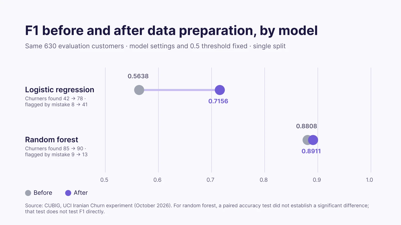
The experiment has clear limits. Under the reported conditions, prepared training data raised F1 for both models, by more for logistic regression.
The results come from one train/test split with 99 churners, and CUBIG did not compare the prepared data against threshold tuning or class weighting on the original data. Retention costs, prevented churn, revenue and workflow time were not measured, and the exported files do not fully document the augmentation algorithm or how every upstream feature-generation step was fitted.
How do you turn churn prediction metrics into a retention decision?
Metrics become a decision once they are expressed as a contact list and its cost. In the logistic regression results from CUBIG’s 2026 experiment, the list grew from 50 to 119 customers: 36 more churners on it, and 33 more customers who did not churn.

A simple way to read that change is incremental net value: the value kept from customers who stay because of the retention action, minus the added contact and incentive costs. The first term counts only the customers the action actually keeps, not every predicted churner who receives an offer, so the team needs an estimate of how often its action works.
Researchers have proposed profit-based metrics for churn models, for example Verbraken, Verbeke and Baesens in IEEE Transactions on Knowledge and Data Engineering (2013). How a team weighs more churners found against more wrong flags in practice is covered in the companion article on customer churn prediction.
| Business situation | Evaluation priority | Why it matters |
|---|---|---|
| Low-cost automated retention messages | Recall | Reaching more churners can justify extra contacts |
| Expensive personalized retention offers | Precision and incremental value | Unnecessary offers use a large share of budget |
| Fixed customer success capacity | Precision at the contact volume the team can handle | Only the top of the list gets contacted |
| High-value subscription contracts | Missed-churn cost within that segment | Losing one large account can outweigh many extra contacts |
| Recurring monthly campaigns | Stability across repeated evaluations | Results need to hold as customer behavior changes |
Writing the chosen row down before the comparison keeps the decision from being made after the numbers are in. For the Iranian Churn experiment those financial outcomes remain unmeasured, so a real team’s next step would be to set the longer list against its budget, its capacity and how often its retention action works.
A random forest that already finds 85 of 99 churners leaves less room to improve, as the same CUBIG experiment (2026) suggested; for that model, a useful next check is whether threshold tuning on the original data reaches a similar result.
CUBIG Shorts
Improved Isn’t the Same as Sufficient
A short take on the question in this section: a model can catch more of what it missed and still miss too many, so agree on the criteria before the numbers come in.
Why does training data matter when a churn model underperforms?
A churn prediction model learns from its training data, so a weak result can come from the data, not only from the algorithm. Missing values, imbalanced classes, inconsistent formats and too few examples of churn all affect what the model learns.
When a churn project underperforms, replacing the model is one response. Another is to check whether the existing data carries enough information to separate customers who leave from those who stay. A dataset with thousands of customers but few churners gives the model far more to learn about customers who stay than about the customers the retention team most needs to find.
Data preparation, such as feature generation or class augmentation, changes those training conditions. A preparation step is not an improvement by default: the step has to be compared against the same prediction objective, under controlled conditions, with measures that show both benefits and trade-offs.
General data quality and fitness for one task are different questions. A dataset can be clean and accessible and still not work for a particular model, evaluation criterion and business objective, and when the data changes again, an earlier evaluation may no longer hold.
Where does Syntitan fit in churn prediction model evaluation?
Syntitan, CUBIG’s AI-ready data platform, prepares and validates enterprise data for a specific AI task and keeps each result as a Version that can be checked again. For churn prediction, the immediate question is often not which new algorithm to choose, but whether the customer data suits the prediction task and whether changing it improves the result under the same evaluation conditions.
Comparing data preparation results with Ready for Model
Ready for Model currently supports binary classification tasks, such as churn or no churn. Syntitan prepares the training data automatically, leaves ID-like key columns and columns it identifies as giving away the answer out of the model inputs, and compares four built-in models (XGBoost, LightGBM, Random Forest and Logistic Regression) before and after preparation on the same evaluation records. The report shows F1, recall, precision and PR-AUC for each model, including results that did not improve.
The comparison shows the effect of data preparation under the tested model settings. The comparison does not show that one model is better in general, or that every preparation step will improve business results.
Making the comparison reproducible
The Proof Kit exports the original and prepared datasets, a run script per model and the split information. In the Iranian Churn experiment, CUBIG reran the exported scripts and reproduced the reported results, which let the team check whether both versions used the same evaluation customers, how many more churners were found, how many false positives were added, and whether ranking improved alongside F1. The Proof Kit reruns model training and scoring; it does not rerun the upstream preparation steps or fully document them.
How does Ready for Model relate to Syntitan’s other checks?
Ready for Raw Data checks a dataset’s general state on six axes (usability, integrity, context, consistency, reproducibility and traceability) without treating one score as fit for every AI task. Ready for Model checks one model task under fixed evaluation conditions. The two answer different questions and do not have to run in order: a good general score does not replace a task-specific comparison, and one successful comparison does not show that a model will stay suitable in production.
Data and AI platforms already cover data preparation, model building and evaluation, so a team may run its own before-and-after tests there. For a team that already builds churn models on such a platform, Ready for Model does not replace the model the team deploys. Ready for Model adds a ready-made before-and-after check, with fixed model settings, the same evaluation records and exported run files, before the team decides how to prepare its own training data. Teams that want their own model compared can ask CUBIG about integration and verification.
Syntitan does not choose the retention offer, deploy the team’s churn prediction model or measure how many customers a campaign keeps; those responsibilities stay with the team that runs the retention workflow.
What should a team check before using an improved churn model?
Before moving a revised churn prediction model into a retention workflow, a team should confirm that the measured improvement is reproducible, relevant to the business objective and practical to act on.
- Prediction objective: what behavior is predicted, over what period, and at what decision point?
- Evaluation consistency: were both versions tested on the same original customers?
- Data readiness: were missing values, available features, class imbalance and possible leakage examined?
- Trade-offs: did recall, precision, F1 and ranking metrics improve or get worse?
- Operational impact: how many more customers would the retention team contact?
- Business value: is there evidence that the extra contacts produce incremental retained value?
- Reproducibility: can the team identify the data, model settings, evaluation conditions and changes behind the result?
If these questions remain open, a higher score is not enough evidence to expand a retention campaign. Once they are answered, the decision may be to proceed, to refine and retest, or to keep the current approach. Model evaluation and data evaluation work together: a team needs to know whether its training data supports the prediction task, which changes help or hurt, and whether those results hold under the conditions where the model will run.
Try it on your data in Syntitan, or run a sample proof with Ready for Model’s sample data before using your own.